by Sony
An open source software to make research,
development and implementation of neural network more efficient.

Features
-
Write less do more
Neural Network Libraries allows you to define a computation graph (neural network) intuitively with less amount of code.
-
Dynamic computation graph support
Dynamic computation graph used enables flexible runtime network construction. The Library can use both paradigms of static and dynamic graph.
-
Run anywhere
We develop the Library by keeping portability in mind. We run CIs for Linux and Windows.
-
Device ready
Most of the code of the Library is written in C++14. By using C++14 core API, you could deploy it onto embedded devices.
-
Easy to add a new function
We have a nice function abstraction as well as a code template generator for writing a new function. Those allow developers write a new function with less coding.
-
Multi-target device acceleration as plugin
A new device code can be added as a plugin without any modification of the Library code. CUDA is actually implemented as a plugin extension.
Products with Sony’s Deep Learning
-

Real Estate Price Estimate
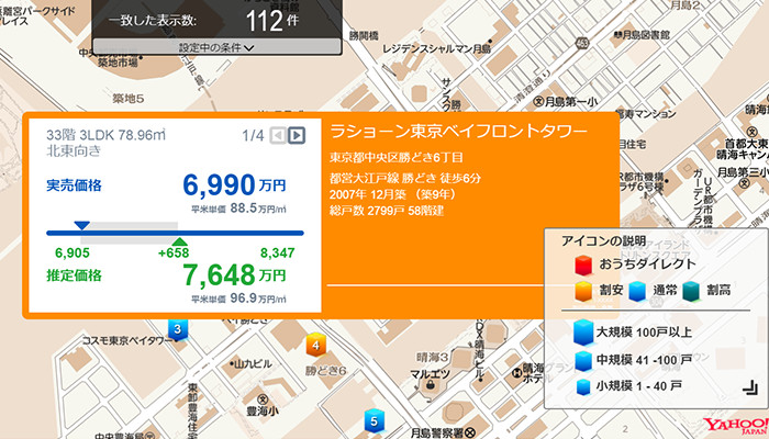
Neural Network Libraries is used in Real Estate Price Estimate Engine of Sony Real Estate Corporation. the Library realizes the solution that statistically estimates signed price in buying and selling real estate, analyzing massive data with unique algorism developed based on evaluation know-how and knowledge of Sony Real Estate Corporation. The solution is utilized in various businesses of Sony Real Estate Corporation such as ”Ouchi Direct”, “Real Estate Property Search Map” and “Automatic Evaluation”.
-

Gesture Sensitivity
The Library is used in an intuitive gesture sensitivity function of Sony Mobile Communications “Xperia Ear”. Based on data from several sensors embedded in Xperia Ear, you can just use a nod of the head to confirm a command - answering Yes/No, answering/declining the phone call, cancelling text-to-speech reading of notifications, skipping/rewinding a song track.
-

Image Recognition (User Identification, Face Tracking, etc.)
The Library is used to realize image recognition of Sony’s Entertainment Robot "aibo" 『ERS-1000』. In the image recognition through fish-eye cameras installed at the nose, the Library is actively utilized for user identification, face tracking, charge stand recognition, generic object recognition, etc. These features and various inbuilt sensors enable its adaptable behavior.
Write Less Do More
You can define a computation graph (neural network) intuitively with less amount of code.
Defining a two layered neural network with softmax loss only requires the following simple 5 lines of code.
x = nn.Variable(input_shape)
t = nn.Variable(target_shape)
h = F.tanh(PF.affine(x, hidden_size, name='affine1'))
y = PF.affine(h, target_size, name='affine2')
loss = F.mean(F.softmax_cross_entropy(y, t))
forward/backward call executes the computation graph.
x.d = some_data
t.d = some_target
loss.forward()
loss.backward()
Parameter management system called parameter_scope enables flexible parameter sharing.
The following code block demonstrates how we write a simple Elman recurrent neural network.
h = h0 = nn.Variable(hidden_shape)
x_list = [nn.Variable(input_shape) for i in range(input_length)]
for x in x_list:
    # parameter scopes are reused over loop,
    # which means parameters are shared for all iteration.
    with nn.parameter_scope('rnn_cell'):
        h = F.tanh(PF.affine(F.concatenate(x, h, axis=1), hidden_size))

y = PF.affine(h, target_size, name='affine')
Dynamic Computation Graph Support
Static computation graph which has been used in general is a method to build a computation graph before executing the graph. On the other hand, dynamic computation graph enables flexible runtime network construction. The Library can use both paradigms of static and dynamic graph. Here is a dynamic computation graph example in the Library.
x = nn.Variable(input_shape)
x.d = some_data
t = nn.Variable(target_shape)
t.d = some_target

with nn.auto_forward():
    h = F.relu(PF.convolution(x, hidden_size, (3, 3), pad=(1, 1), name='conv0'))
    for i in range(num_stochatic_layers):
        if np.random.rand() < layer_drop_ratio:
            continue  # Stochastically drop a layer.
        h2 = F.relu(PF.convolution(x, hidden_size, (3, 3), pad=(1, 1),
                                   name='conv%d' % (i + 1)))
        h = F.add2(h, h2)
    y = PF.affine(h, target_size, name='classification')
    loss = F.mean(F.softmax_cross_entropy(y, t))

# Backward computation can also be done in dynamically executed graph.
loss.backward()
The memory caching system implemented in the Library enables fast execution without memory allocation overhead.
Ready for More?
We have just briefly introduced the most basic features of the Library. Docs will cover them and other advanced features with much finer details, so make sure to read through it all!!!!
The New Deep Learning Experience
Neural Network Console
Not just train and evaluate.
You can design neural networks with fast and intuitive GUI.